MMVFree - User Guide

© 2026 Medicines for Malaria Venture. All rights reserved.

Cite this guide

Introduction

MMVFree is a web tool for multi-compound dose prediction of malaria drug candidates, formulating dose criteria based on free (unbound) drug concentrations. For each compound, it predicts the dose required for the unbound plasma concentration to stay above the unbound minimum inhibitory concentration (MIC_u - the unbound concentration below which the parasite population is no longer fully suppressed) for a specified duration, for both an oral and a long-acting injectable (LAI) route of administration. Predictions are derived directly from in vitro intrinsic clearance and potency data together with a volume of distribution (Vss, used throughout in its unbound form, Vss_u) estimate - no in vivo human data and no PK/PD concentration-time simulation are required. This makes MMVFree faster and lighter-weight than the sibling app MMVSola, at the cost of some of the modelling detail MMVSola provides (e.g. MMVSola simulates full PK/PD profiles and supports multi-species IVIVE scaling from hepatocyte data; MMVFree works from a microsomal intrinsic clearance measurement and a well-stirred liver model based hepatic extraction correction - see Chapter 2).

Input → Unbound Parameters & Dose

MMVFree’s workflow is organized around two tabs:

File Input. The user uploads a Science Cloud database extract or a previously generated MMVFree report (Excel format) containing, for one or more compounds: molecular weight, blood plasma ratio, human plasma/Albumax/microsomal % binding, SMILES code, in silico and/or in vivo (rat) Vss, in vitro TCGLS 3D7 72h IC50, in vitro parasite reduction ratio (PRR) and PRR lag time, and microsomal intrinsic clearance. When several measurements exist for the same parameter (e.g. assay replicates), they are averaged - the user can review and exclude individual records from this averaging, and can overwrite any value manually. Missing values fall back to documented defaults where possible. A Science Cloud upload isn’t required either - every one of these parameters can instead be typed directly into the Input Parameters table for a compound with no uploaded data at all (Chapter 1, Step 2).

Unbound Parameters & Dose. This tab is populated automatically once compound data is available, and lets the user set the oral (target duration, number of doses, dosing interval) and LAI (90- or 180-day coverage) prediction settings from the sidebar. It shows, for every compound and for both an in silico and an in vivo Vss estimate, the predicted unbound PK parameters (Chapter 2) and predicted doses (Chapter 3), split into three sections - unbound parameters, oral dose, and LAI dose - each dose section pairing a compact table with a dose-landscape plot. Each dose table row also links out to the sibling MMVSola and LAI Parameter Explorer apps with as many parameters pre-filled as MMVFree can supply (Chapter 1). A Report button in the sidebar downloads a multi-sheet Excel workbook documenting the inputs and predictions (see Chapter 4); a previously generated MMVFree report can itself be re-uploaded on the File Input tab, making it easy to resume earlier work or combine results across sessions.

This guide first walks through a practical usage scenario (Chapter 1), then describes the underlying methods - unbound PK parameter prediction (Chapter 2) and dose prediction (Chapter 3) - and finally explains what the downloadable report contains (Chapter 4).

1 Quick Start

This chapter walks through a complete MMVFree session for a single compound: uploading data, reviewing the predicted parameters and doses, downloading a report, and jumping across to the sibling apps MMVSola and LAI Parameter Explorer for a compound of interest. It uses the malaria drug chloroquine (tests/testthat/MMV008_Chloroquine.xlsx in the MMVFree repository) as a worked, non-confidential example throughout.

A tip before you start: if a screenshot below looks too small to read, right-click it and choose Open image in new tab (or your browser’s equivalent) to view it at full resolution.

Before you start: export the data from Science Cloud

In Science Cloud, select your compounds and batches, click Export above the results table (Figure 1.1), choose RD-00-0000 - GENERIC MMVSOLA EXTRACTION on the Standard tab and click Export again (Figure 1.2). The Excel file this produces is the Science Cloud extract uploaded in Step 1.

Figure 1.1: The Export button in the Science Cloud search results

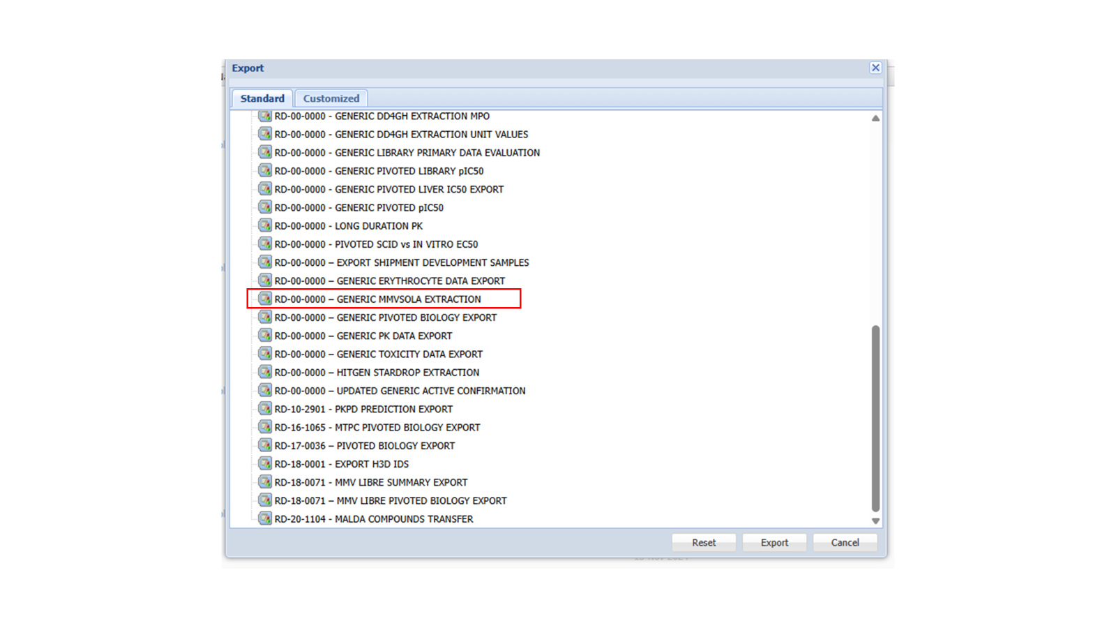
Figure 1.2: The Science Cloud export dialog with the extraction to select highlighted

Step 1: Upload a Science Cloud file

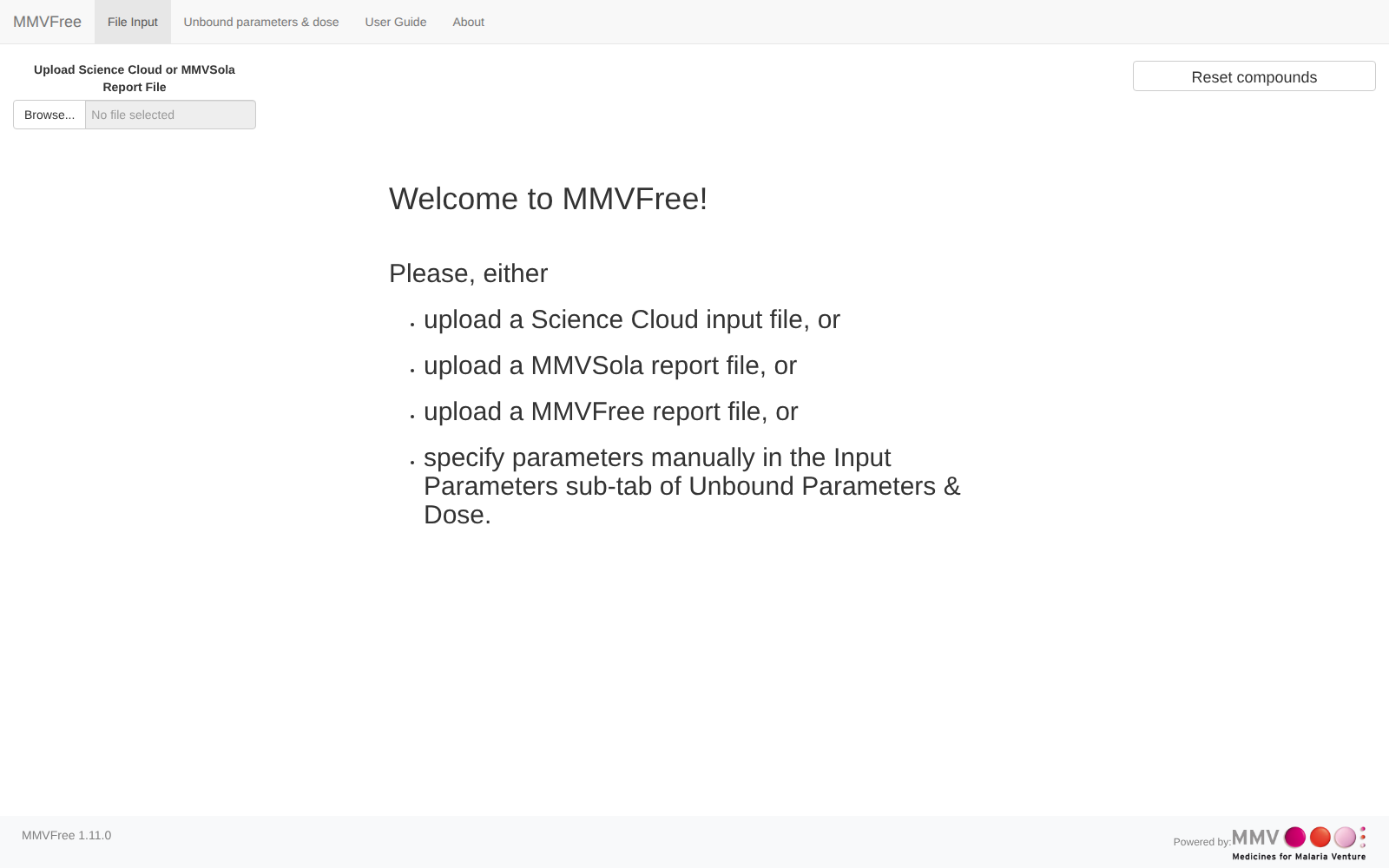
MMVFree opens on the File Input tab. Before anything is uploaded, it shows a short welcome message listing the ways to get started - a Science Cloud extract, a previously generated MMVSola or MMVFree report, or entering parameters manually. (“Entering parameters manually” means skipping this step entirely and instead typing values directly into the Input Parameters table - see Step 2 below.)

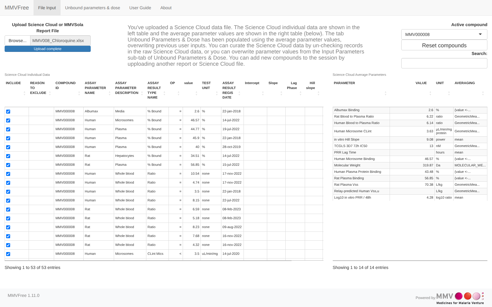
Click Browse… and select a Science Cloud Excel export (or a prior MMVFree/MMVSola report - see Chapter 4 for what a report contains). Once uploaded, the File Input tab shows two tables: Science Cloud Individual Data on the left - every raw assay record for the compound, with a checkbox to include or exclude each one from averaging - and Science Cloud Average Parameters on the right, the averaged value MMVFree actually uses for each parameter, together with its unit and the averaging method applied.

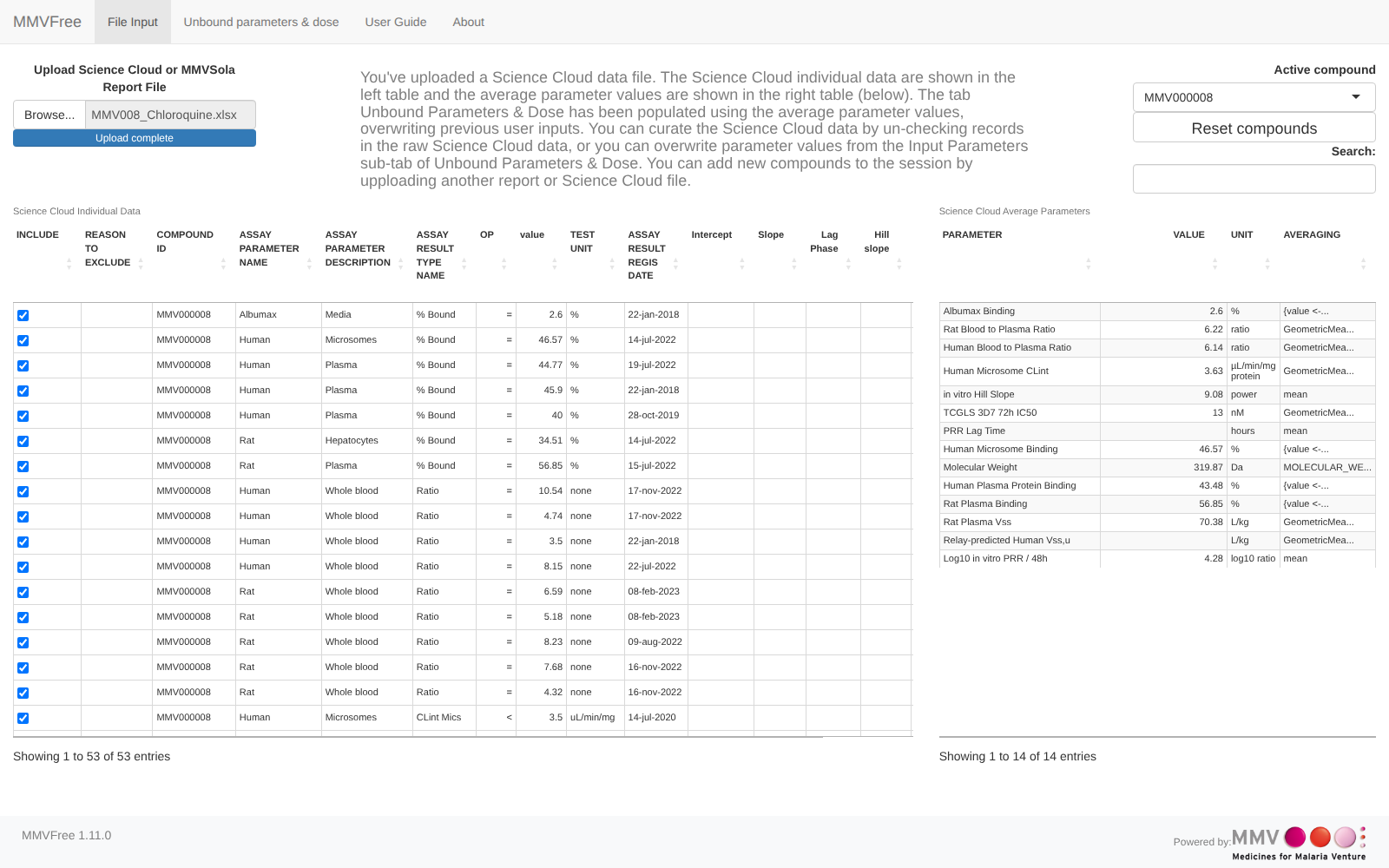
When more than one compound has been loaded, the Active compound selector (top right) chooses which compound’s two tables are displayed - it stays in sync with the compound selected anywhere else in the app (see the cross-table highlighting mentioned in the next step). Unchecking a record in the left-hand table live-recalculates that compound’s averaged values without needing to re-upload the file.

Step 2: Review the aggregated Input Parameters

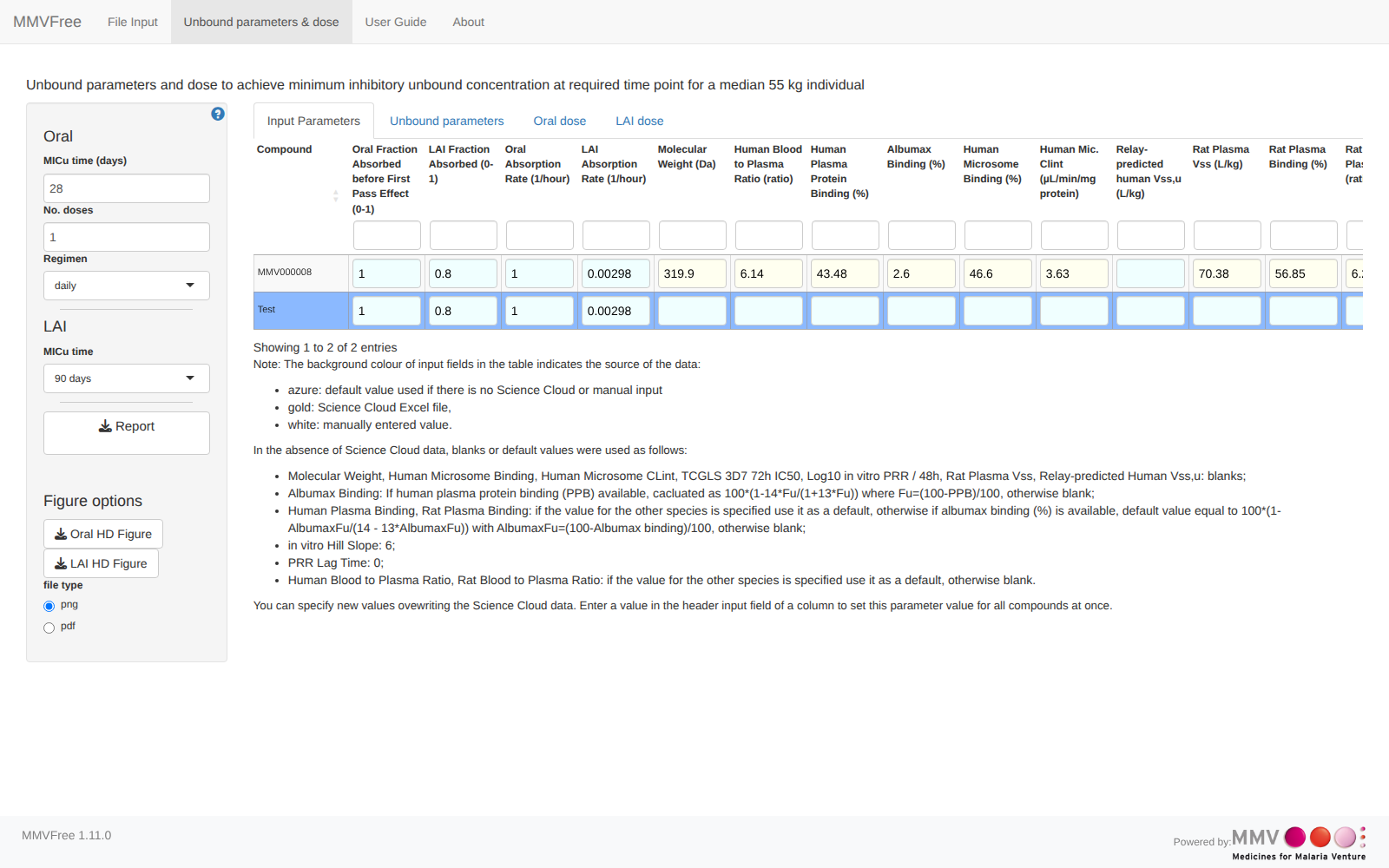
Switch to the Unbound parameters & dose tab. Its Input Parameters sub-tab (open by default) shows one row per compound with every input parameter MMVFree found or defaulted - color-coded by source (gold: from the Science Cloud file; white: entered/overwritten manually; azure: a built-in default used because no value was available).

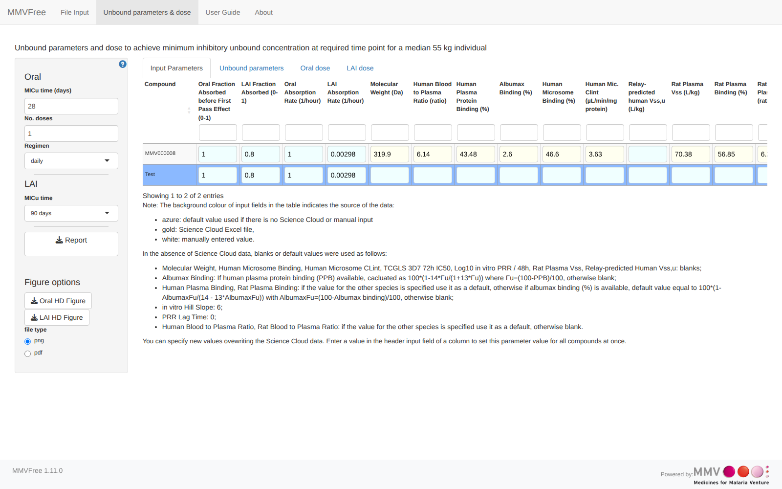
Clicking a compound’s row here (or in any of the three tables in the steps below) highlights that same compound everywhere else in the app - the other tables, the dose-landscape plots, and the File Input tab’s Active compound selector all follow along.

You can overwrite any cell directly, or type a value into a column’s header input field to apply it to every compound at once.

Step 3: Read the predicted unbound parameters

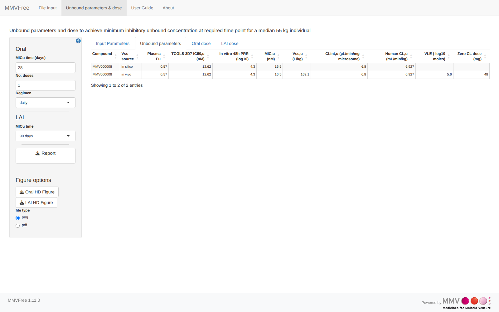
The Unbound parameters sub-tab shows the PK parameters MMVFree derives from the inputs above - unbound intrinsic clearance, unbound volume of distribution (from two independent estimates, “Vss source”), elimination rate and half-life, and unbound potency (MIC_u). Chapter 2 explains exactly how each column is derived.

Step 4: Read the Oral dose prediction

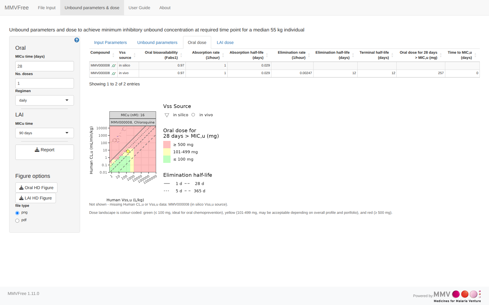
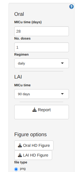
The Oral dose sub-tab predicts the dose needed to keep the unbound concentration above MIC_u for the target you set in the sidebar - MICu time (days), No. doses, and Regimen (daily/weekly/monthly). The table shows one row per Vss source; the dose-landscape plot below it overlays the compound’s two predicted points on a theoretical grid across a wide range of hypothetical Vss_u/CL_int,u combinations, colour-coded by dose category (see the footnote under the plot for the exact thresholds). Chapter 3 covers the underlying dose formula and how to read the landscape plot in full.

Step 5: Read the LAI dose prediction

The LAI dose sub-tab is the long-acting-injectable equivalent, targeting the coverage duration selected in the sidebar’s MICu time control (90 or 180 days). A single administration is assumed, so there is no “No. doses”/“Regimen” control for this route.

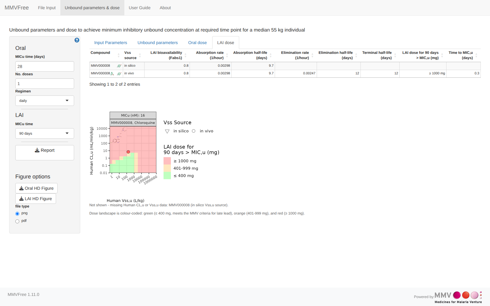
The sidebar controls relevant to both dose sub-tabs are grouped together, alongside the Report button used in the next step:

Step 6: Download the report

Click Report in the sidebar to download a multi-sheet Excel workbook documenting the uploaded inputs and every prediction shown above, for every loaded compound. Chapter 4 describes what each of its 7 sheets contains. A report downloaded this way can itself be re-uploaded later on the File Input tab (Step 1), making it easy to resume a session or combine results from several uploads.

Step 7: Explore a compound in MMVSola or LAI Parameter Explorer

Each row of the Oral dose and LAI dose tables carries small link icons next to the compound name, for jumping to two sibling MMV applications with as many parameters pre-filled as MMVFree can supply - saving the manual re-entry of everything MMVFree already knows about the compound.

• The MMVSola icon (a green molecule glyph) appears on both the Oral dose and LAI dose sub-tabs. Clicking it opens MMVSola in a new tab, landing on the matching Prediction sub-tab (Oral or LAI) with the compound’s name and every transferable parameter already filled in.
• The LAI Parameter Explorer icon appears only on the LAI dose sub-tab (an oral MMVFree compound has no direct LAI Parameter Explorer equivalent to link to). Clicking it opens LAI Parameter Explorer with the same pre-fill behavior.

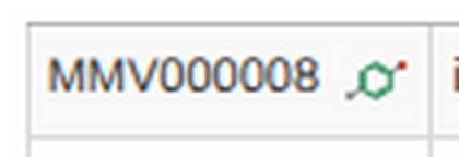
Figure 1.3: The MMVSola link icon on the Oral dose sub-tab (Compound column)

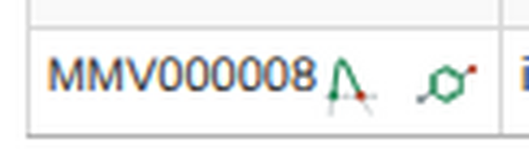
Figure 1.4: Both link icons on the LAI dose sub-tab: LAI Parameter Explorer (left) and MMVSola (right)

Following the MMVSola icon from the Oral dose row above opens MMVSola already on its Oral Prediction sub-tab, with the compound field validated (green checkmark) and the transferred parameters - molecular weight, plasma binding, blood-to-plasma ratio, in vitro clearance and potency, Vss, and oral absorption - already populating its own prediction, with no further input needed:

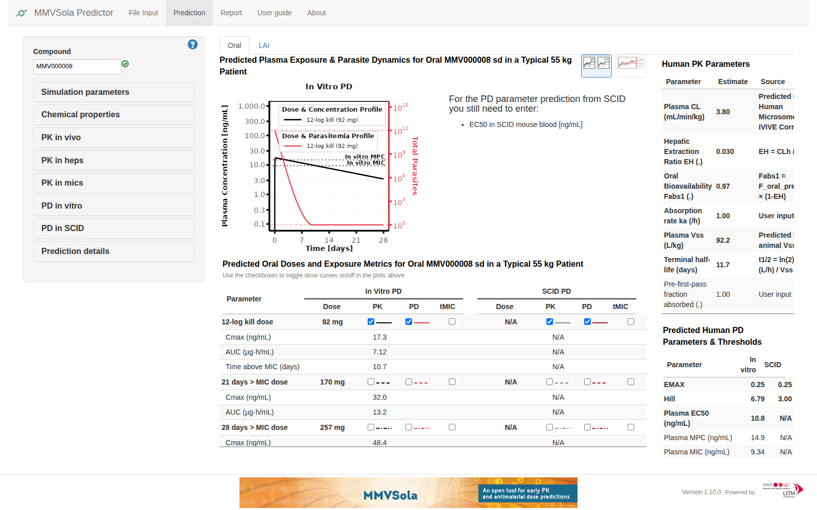
Figure 1.5: MMVSola’s Oral Prediction sub-tab immediately after following the link from MMVFree

A row missing a parameter a destination app requires for its own link gets no icon for that destination at all, rather than a link with a blank or “NA” value in it - so an icon’s absence is itself informative: something that row needs is missing further up in the File Input or Input Parameters step.

2 Unbound Parameter Prediction

2.1 Overview

For every compound, MMVFree predicts a small set of unbound (free-drug) PK parameters - unbound intrinsic clearance, unbound volume of distribution, and unbound potency (MIC_u) - directly from in vitro clearance/potency data and a volume-of-distribution estimate (the elimination rate and terminal half-life are also estimated from these same inputs). These parameters are what the dose predictions of Chapter 3 are built from. All patient-scale quantities use a fixed reference body weight of 55 kg.

The diagram below is a map of how those predictions are derived: boxes are quantities, arrows are derivation steps, and arrow labels name the assumption or method behind each step. It collapses into three independent chains that only meet at \(k_e\) and \(F_h\): clearance and hepatic extraction (left - \(CL_{int,u}\) is itself a reported output, “Human CL,u”, not just an intermediate), which feeds both \(k_e\) (together with volume of distribution) and, via \(F_h\), oral bioavailability \(F\) (together with the Oral Fraction Absorbed input - used by the dose formula in Chapter 3); and two chains that don’t touch the rest at all - LAI terminal half-life (set entirely by the fixed LAI absorption rate \(k_{a,LAI}\), not by clearance or volume) and unbound potency, MIC_u (its own in vitro-to-human chain, described in 2.7). The oral terminal half-life additionally depends directly on \(k_{a,oral}\) (via the “\(k_{a,oral} \gg k_e\)” rate-limiting condition), not just on \(k_e\). Blue boxes are inputs (measured or otherwise supplied), grey boxes are intermediates, green boxes are this chapter’s outputs (some, like \(CL_{int,u}\), are both).

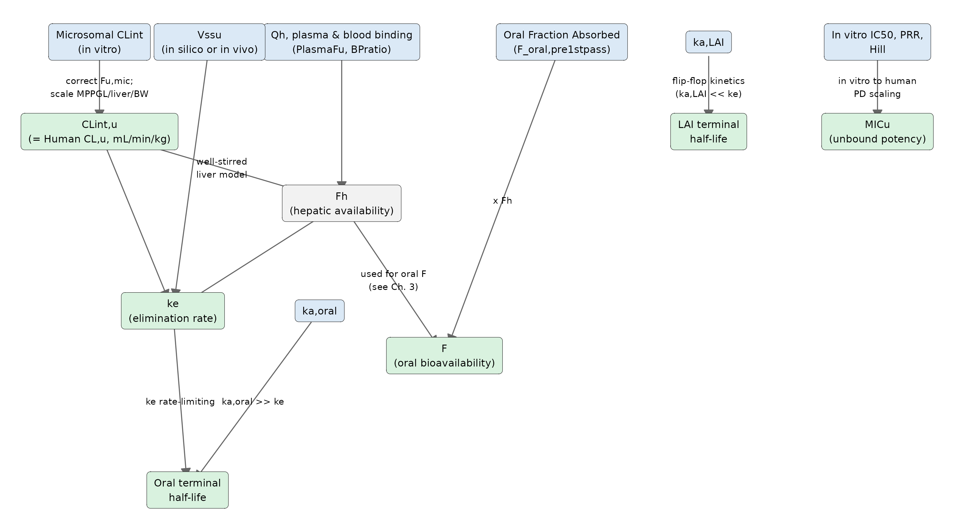
The sections below walk through each of these steps in full, in the order: unbound intrinsic clearance (2.2), volume of distribution (2.3), hepatic extraction and \(k_e\) (2.4, 2.5), terminal half-life (2.6), and unbound potency (2.7).

Several of the quantities in the diagram look similar but are defined in different matrices - blood, plasma, or an in vitro assay medium - and some of those also come in a total (bound + unbound) and an unbound (free) form within the same matrix. Mixing either of these up is the easiest way to misread a PK formula. The glossary below lists every symbol used in this chapter, together with its Kind - whether it’s an Input (a value the user supplies, directly or via an uploaded file), a Constant (a fixed value built into MMVFree, not compound-specific), or Derived (calculated from other quantities in this table, via the formula shown) - for reference while reading the sections that follow.

Symbol	Kind	Meaning	Matrix	Typical units
BW	Constant	Reference body weight \(=55\)	-	kg
MPPGL	Constant	Microsomal protein per gram liver \(=40\) (updated 2026-06-18, MMVFree#5)	-	mg protein/g liver
LiverWeight	Constant	Human liver weight \(=25.5\) (updated 2026-06-18, MMVFree#5)	-	g liver/kg BW
\(Q_h\)	Constant	Hepatic blood flow \(=20.7\) (MMVbase::get_NumericConstantsAsList()$QhPatient_mLPerMinPerkg)	Blood	mL/min/kg
\(CL_{int,mic}\)	Input	Measured microsomal intrinsic clearance (total, not yet corrected for microsomal binding)	In vitro	µL/min/mg protein
BPratio	Input	Blood-to-plasma concentration ratio	Relates blood ↔︎ plasma	-
\(Vss\)	Input	Steady-state volume of distribution, total - as conventionally measured (e.g. rat \(Vss_R\))	Plasma	L/kg
\(k_{a,oral}\), \(k_{a,LAI}\)	Input	Absorption rate constants (oral / LAI)	-	1/h
\(F_{oral,pre1stpass}\)	Input	Oral fraction absorbed before first-pass extraction	-	- (0-1)
\(IC50\)	Input	In vitro potency, total (bound)	In vitro	nM
\(Fu_{mic}\)	Derived	Fraction of drug unbound in the microsomal incubation (\(=1-\%\text{MicrosomePB}/100\))	In vitro	-
\(CL_{int,u}\)	Derived	Unbound, whole-body-scaled intrinsic clearance - reported in the app as “Human CL,u”	Intrinsic - not tied to a blood or plasma matrix, see 2.2	L/h or mL/min/kg
\(Fu_{plasma}\)	Derived	Fraction of drug unbound in plasma (\(=1-\%\text{PPB}/100\))	Plasma	-
\(Fu_b\)	Derived	Fraction of drug unbound in blood (\(=Fu_{plasma}/\text{BPratio}\))	Blood	-
\(C_{in}\), \(C_{out}\)	Derived	Drug concentration in blood entering / leaving the liver (conceptual, well-stirred model derivation only)	Blood	mg/L
\(CL_h\)	Derived	Hepatic clearance from the well-stirred model	Blood	mL/min/kg
\(E_H\)	Derived	Hepatic extraction ratio (\(=CL_h/Q_h\))	Blood	-
\(F_h\)	Derived	Hepatic availability factor: fraction surviving one pass through the liver (\(=1-E_H\))	-	- (0-1)
\(CL_{plasma}\)	Derived	Hepatic clearance re-expressed in the plasma matrix, total (\(=CL_h \times \text{BPratio}\))	Plasma	mL/min/kg
\(Vss_u\)	Derived	Unbound volume of distribution (\(=Vss/Fu_{plasma}\))	Plasma	L or L/kg
\(k_e\)	Derived	Elimination rate constant	-	1/h
\(F\)	Derived	Oral bioavailability (\(=F_{oral,pre1stpass} \times F_h\)) - used by the dose formula, Chapter 3	-	- (0-1)
\(Fu_{Albumax}\)	Derived	Fraction of drug unbound in the Albumax-supplemented in vitro assay medium (\(=1-\%\text{AlbumaxPB}/100\))	In vitro	-
\(IC50_u\)	Derived	In vitro potency, unbound (\(=IC50 \times Fu_{Albumax}\))	In vitro	nM
\(MIC_{plasma}\)	Derived	Minimum inhibitory concentration, total	Plasma	ng/mL
\(MIC_u\)	Derived	Unbound minimum inhibitory concentration	Plasma	nM

\(CL_{int,u}\) isn’t tied to a blood or plasma matrix, because intrinsic clearance is defined at the level of the liver’s enzymes acting on unbound drug, before any question of how that drug is carried in blood or plasma arises - the blood/plasma distinction only enters once whole-organ blood flow (\(Q_h\)) gets involved, in the hepatic extraction model below.

2.2 Unbound Intrinsic Clearance (CL_int,u)

The starting point is a measured microsomal intrinsic clearance, CLint_mic_H_uLminmg (µL/min/mg microsomal protein) - a total, uncorrected in vitro measurement, since the incubation itself involves some degree of microsomal protein binding. MMVFree reports two related but distinct unbound clearance values derived from it, at two different scales:

1. Unbound intrinsic clearance at assay scale. Dividing directly by the fraction unbound in the microsomal incubation, \(Fu_{mic}\), gives the unbound clearance still expressed per mg of microsomal protein - reported in the app as “CL_int,u (µL/min/mg microsome)”:

\[CL_{int,u,mic} \; [\mu L/min/mg] = \frac{CL_{int,mic}}{Fu_{mic}}, \qquad Fu_{mic} = 1 - \frac{\%\text{MicrosomePB}}{100}\]

2. Unbound intrinsic clearance at whole-body scale. This is obtained by, first, scaling the total (not yet fu-corrected) \(CL_{int,mic}\) to a whole-body total clearance using microsomal protein per gram of liver (MPPGL) and liver weight per kg body weight (Obach 1999; Houston 1994) and converting µL/min/mg protein to L/h for the reference patient:

\[CL_{int} \; [\text{L/h}] = CL_{int,mic} \times 10^{-6} \times 60 \times \text{MPPGL} \times \text{LiverWeight} \times \text{BW}\]

where (see the Symbol Glossary above) \(\text{MPPGL} = 40\) mg protein/g liver and \(\text{LiverWeight} = 25.5\) g liver/kg body weight, then dividing by the same \(Fu_{mic}\) as step 1, to get the unbound whole-body intrinsic clearance. This reuses a single \(Fu_{mic}\), measured once in the in vitro incubation, for both steps - implicitly assuming that fraction unbound also holds for the liver’s own microsomal protein environment, not just the assay’s:

\[CL_{int,u} \; [\text{L/h}] = \frac{CL_{int} \; [\text{L/h}]}{Fu_{mic}}\]

converted to mL/min/kg for reporting and for the hepatic extraction model below:

\[CL_{int,u} \; [\text{mL/min/kg}] = CL_{int,u} \; [\text{L/h}] \times \frac{1000}{60 \times \text{BW}}\]

reported in the app as “Human CL,u (mL/min/kg)”. It is this whole-body value, \(CL_{int,u}\), that feeds the hepatic extraction model in the next section.

2.3 Volume of Distribution (Vss_u)

Two independent unbound \(Vss_u\) estimates are used per compound, both scaled to the 55 kg reference body weight:

• In silico: a relay-predicted human unbound \(Vss_u\) per kg - not computed by MMVFree itself, but an input value typically populated from Science Cloud, or entered manually. It’s scaled directly by body weight; since the input is already unbound, no further fu correction is needed here.
• In vivo: allometrically scaled by MMVFree from a measured rat volume of distribution, \(Vss_R\) (the conventional, total volume of distribution, in the plasma matrix), correcting for rat plasma protein binding to convert it to the same unbound form as the in silico estimate:

\[Vss_{u,\text{in vivo}} = \frac{Vss_{R} \; [\text{L/kg}]}{Fu_{plasma,R}} \times \text{BW}\]

Every downstream parameter that depends on \(Vss_u\) (elimination rate, half-life, dose) is therefore computed twice per compound - once from each estimate - and both are shown on separate rows in the app’s output tables, labelled by “Vss source”.

2.4 Hepatic Extraction and Bioavailability (F_h)

2.4.1 The Well-Stirred Model

The well-stirred liver model (also called the venous equilibration model) is the standard way to describe hepatic drug elimination, treating the liver as a single, well-mixed compartment (Rowland, Benet, and Graham 1973). It rests on three assumptions:

1. Instantaneous mixing: blood entering the liver is immediately and perfectly mixed with liver tissue, so the drug concentration throughout the liver equals the concentration in the emerging hepatic vein, \(C_{out}\). This requires reasonable membrane permeability and no significant role of hepatic efflux transporters.
2. Only unbound drug is eliminated: entry into hepatocytes is not rate-limiting; only unbound (free) drug can cross the hepatocyte membrane to reach the metabolizing enzymes.
3. Linear kinetics: elimination is first-order, so \(CL_{int,u}\) is constant regardless of drug concentration.

Note: for low-clearance compounds, the well-stirred model is equivalent to other liver models. Hepatic metabolism is treated as the only clearance mechanism considered.

A note on notation. Textbook derivations of the well-stirred model are usually written in terms of a generic clearance term, often just labelled “CL” - but what actually enters this derivation is \(CL_{int,u}\), the unbound intrinsic clearance derived above (2.2): the enzymes’ own capacity to remove unbound drug, independent of blood flow or protein binding. \(CL_h\) and \(CL_{plasma}\), derived below, are the whole-organ clearances that come out of this derivation - conceptually downstream of \(CL_{int,u}\), not the same quantity as it.

Deriving the extraction ratio. The hepatic extraction ratio, \(E_H\), is the fraction of drug removed from the blood during a single pass through the liver, defined directly from the concentrations entering and leaving the organ, \(C_{in}\) and \(C_{out}\):

\[E_H = \frac{C_{in} - C_{out}}{C_{in}}\]

To connect this basic definition to \(Fu_b\) and \(CL_{int,u}\), apply mass balance together with the well-stirred assumption:

1. Mass balance: the rate of drug entering the liver equals the rate leaving plus the rate eliminated inside it (Rowland and Tozer 2022): \[Q_h \cdot C_{in} = Q_h \cdot C_{out} + \text{Rate of elimination} \quad\Rightarrow\quad \text{Rate of elimination} = Q_h \cdot (C_{in} - C_{out})\]
2. Enzymatic rate: only unbound drug is eliminated, at a rate set by \(CL_{int,u}\) and the unbound concentration at the enzyme site, \(C_{u,liver}\): \[\text{Rate of elimination} = CL_{int,u} \cdot C_{u,liver}\]
3. Well-stirred assumption: \(C_{u,liver}\) is in instantaneous equilibrium with the unbound concentration in the exiting blood, \(C_{u,liver} = Fu_b \cdot C_{out}\), so: \[\text{Rate of elimination} = Fu_b \cdot CL_{int,u} \cdot C_{out}\]
4. Solve for \(E_H\): the two expressions for the rate of elimination (steps 1 and 3) describe the same thing, so they’re equal: \[Q_h \cdot (C_{in} - C_{out}) = Fu_b \cdot CL_{int,u} \cdot C_{out}\] Dividing both sides by \(C_{in}\) and writing \(C_{out}/C_{in} = 1 - E_H\) gives \(Q_h \cdot E_H = Fu_b \cdot CL_{int,u} \cdot (1-E_H)\); solving this for \(E_H\): \[E_H = \frac{Fu_b \cdot CL_{int,u}}{Q_h + Fu_b \cdot CL_{int,u}}\]

Fraction surviving first-pass (\(F_h\)), the fraction of drug that escapes hepatic extraction and reaches systemic circulation: \(F_h = 1 - E_H\), so:

\[F_h = \frac{Q_h}{Q_h + Fu_b \cdot CL_{int,u}}\]

Hepatic clearance (\(CL_h\)), the volume of blood fully cleared of drug per unit time, is by definition \(CL_h = Q_h \cdot E_H\). Substituting the \(E_H\) formula above gives the well-stirred model’s clearance equation:

\[CL_h = \frac{Q_h \cdot Fu_b \cdot CL_{int,u}}{Q_h + Fu_b \cdot CL_{int,u}}\]

2.4.2 CL_h in Terms of F_h

\(E_H\), \(F_h\) and \(CL_h\) above all still depend on \(Q_h\). It’s useful to eliminate \(Q_h\) and express \(CL_h\) using only \(Fu_b\), \(CL_{int,u}\), and \(F_h\):

1. Start from \(CL_h = Q_h \cdot E_H = Q_h \cdot (1 - F_h)\).
2. Solve the \(F_h\) formula above for \(Q_h\): \(F_h \cdot (Q_h + Fu_b \cdot CL_{int,u}) = Q_h\), so \(Q_h = \dfrac{F_h \cdot Fu_b \cdot CL_{int,u}}{1 - F_h}\).
3. Substitute into step 1: \(CL_h = \dfrac{F_h \cdot Fu_b \cdot CL_{int,u}}{1 - F_h} \times (1-F_h)\). The \((1-F_h)\) terms cancel, leaving: \[CL_h = Fu_b \cdot CL_{int,u} \cdot F_h\]

Interpretation. This says the actual hepatic clearance is the maximum theoretical enzymatic capability (\(Fu_b \cdot CL_{int,u}\)), scaled down by the fraction of drug that actually reaches the enzymes intact (\(F_h\)) (Gabrielsson and Weiner 2016):

• Low-extraction drug (\(E_H \approx 0\), \(F_h \approx 1\)): \(CL_h \approx Fu_b \cdot CL_{int,u}\)
  • clearance depends only on protein binding and enzyme activity, not blood flow.
• High-extraction drug (\(E_H \approx 1\), \(F_h\) small): \(F_h\) becomes a bottleneck - even a very large \(CL_{int,u}\) can’t push \(CL_h\) much past \(Q_h\), so clearance becomes blood-flow-limited rather than enzyme-limited.

2.4.3 F_h’s Two Roles in MMVFree

\(F_h\) is used in two places in MMVFree, for two different reasons:

• Oral bioavailability: an oral dose passes through the liver once (via the portal vein) before reaching the rest of the body, and \(F_h\) is exactly the fraction that survives that single pass - it multiplies directly into oral \(F\) (Chapter 3). An LAI dose skips this entirely, since intramuscular/subcutaneous injection bypasses the portal vein.
• Elimination rate: \(F_h\) is not a second first-pass loss here - it’s simply part of how \(CL_h\) factors, per \(CL_h = Fu_b \cdot CL_{int,u} \cdot F_h\) above (2.4.2).

2.5 Elimination Rate Constant (k_e)

\[k_e = \frac{CL_{int,u} \cdot F_h}{Vss_u}\]

computed independently for each of the two \(Vss_u\) estimates above (in silico and in vivo), giving two \(k_e\) values per compound. Reported in the app as “Elimination rate (1/hour)”.

Where this comes from. The textbook definition is \(k_e = CL/Vss\), both in the same matrix (plasma, conventionally). Starting from \(CL_h = Fu_b \cdot CL_{int,u} \cdot F_h\) (2.4.2):

1. \(CL_h\) is a blood clearance; converting it to a plasma clearance needs the blood-to-plasma ratio, \(CL_{plasma} = CL_h \times \text{BPratio}\). Substituting \(Fu_b = Fu_{plasma}/ \text{BPratio}\), the BPratio cancels: \(CL_{plasma} = Fu_{plasma} \cdot CL_{int,u} \cdot F_h\).
2. \(Vss_u = Vss/Fu_{plasma}\) (previous section), so \(Vss = Vss_u \cdot Fu_{plasma}\).
3. \(k_e = CL_{plasma}/Vss = \dfrac{Fu_{plasma} \cdot CL_{int,u} \cdot F_h}{Vss_u \cdot Fu_{plasma}} = \dfrac{CL_{int,u} \cdot F_h}{Vss_u}\): \(Fu_{plasma}\) cancels, recovering the app’s formula. Even though \(CL_h\) is built from blood fu and \(Vss_u\) from plasma fu, the two don’t need to match, because step 1 already converts between them.

2.6 Terminal Half-Life

Each route’s dose table reports three separate half-lives, all in days:

• Absorption half-life: \(t_{1/2,abs} = \ln(2) / k_a\), using the route’s own absorption rate (\(k_{a,oral}\), default 1/h, or \(k_{a,LAI}\), default \(2.98 \times 10^{-3}\)/h - the estimated absorption rate of medroxyprogesterone acetate, the fastest-absorbing intramuscular aqueous suspension known). Route-specific, but the same for both Vss sources of a given compound (it doesn’t depend on \(Vss_u\) or clearance at all).
• Elimination half-life: \(t_{1/2,elim} = \ln(2) / k_e\), using the route-independent \(k_e\) from the previous section. The same value feeds both the Oral dose and LAI dose tables.
• Terminal half-life: the half-life that actually governs the terminal (long-time) phase of the concentration-time curve - set by whichever of absorption or elimination is slower (“rate-limiting”) for that route: \(t_{1/2,term} = \ln(2) / \min(k_a, k_e)\).

Where \(\min(k_a, k_e)\) comes from. Chapter 3’s single-dose concentration curve (3.2.1) is a difference of two exponentials: \[C_1(t) = \frac{F \cdot Dose \cdot k_a}{Vss \cdot (k_a - k_e)} \left(e^{-k_e t} - e^{-k_a t}\right)\] At large \(t\), whichever of \(e^{-k_e t}\) or \(e^{-k_a t}\) has the larger rate constant decays to zero first, leaving the other term to dominate the curve - so for large \(t\), \(C_1(t) \approx \text{const} \times e^{-\min(k_a,k_e) \, t}\). The terminal phase is therefore a simple, single exponential decline governed by whichever rate is smaller (slower) - the rate-limiting one - giving the terminal half-life \(t_{1/2,term} = \ln(2) / \min(k_a, k_e)\) above.

Oral usually has \(k_{a,oral} \gg k_e\), so its terminal half-life usually equals the elimination half-life; LAI usually has \(k_{a,LAI} \ll k_e\) (“flip-flop” kinetics), so its terminal half-life usually equals the absorption half-life and is essentially fixed across compounds. Both are only the usual case, though - MMVFree computes the actual \(\min(k_{a,oral}, k_e)\) and \(\min(k_{a,LAI}, k_e)\) per compound rather than assuming which rate applies by route, so an atypical compound (e.g. unusually slow oral absorption, or unusually slow elimination) can have its terminal half-life governed by the other rate instead, for either route.

2.7 Unbound Potency (MIC_u)

Potency is predicted from in vitro assay data via the following chain:

1. Unbound IC50: \(IC50_u = IC50 \times Fu_{Albumax}\), correcting the assay IC50 for binding in the Albumax-supplemented in vitro growth medium.
2. E_max: derived from the in vitro 48h parasite reduction ratio (PRR) via the parasite growth rate observed in vitro.
3. Human blood EC50 and Hill coefficient: predicted from the in vitro IC50/PRR/Hill inputs, correcting for plasma and Albumax binding, blood-to-plasma ratio, and molecular weight.
4. Minimum inhibitory concentration: solved from the E_max model at the in vivo parasite growth rate, then divided by BPratio to convert from blood to plasma concentration.
5. MIC_u: the plasma MIC converted to unbound, nM units: \[MIC_u \; [\text{nM}] = MIC_{plasma} \; [\text{ng/mL}] \times Fu_{plasma} \times \frac{1000}{MW}\]

2.8 Supplementary Diagnostics

Two additional derived quantities are shown for reference, not used directly in dose prediction:

• VLE (volume-ligand efficiency, \(-\log_{10}\) moles): \(VLE = -\log_{10}(MIC_u/10^9) - \log_{10}(Vss_u / BW)\), a potency/distribution efficiency metric independent of clearance.
• Zero CL dose: the hypothetical dose that would be needed to reach \(MIC_u\) if the compound had zero clearance, \(= MIC_u \; [\text{mg/L}] \times Vss_u \; [\text{L}]\) - a lower bound on achievable dose, useful for sanity-checking predictions dominated by a very high clearance.

3 Dose Prediction

3.1 Dose Criterion

For both routes, MMVFree predicts the smallest dose for which the unbound plasma concentration stays at or above MIC_u (Chapter 2) continuously for a user-specified duration - counted as a continuous window that must last at least that long, starting from whenever concentration first reaches MIC_u (its onset), not from a fixed, dose-independent point in time such as the end of the dosing regimen. The two routes differ in how that duration and dosing regimen are specified:

• Oral: a target duration (“MICu time”, in days), a number of doses, and a dosing interval (daily/weekly/monthly) are all user-configurable in the sidebar.
• LAI: a single administration is assumed (one dose, no repeat interval), for a user-selected target duration of either 90 or 180 days.

3.2 How the Dose Is Predicted

3.2.1 The Assumed PK Model

MMVFree assumes a one-compartment model with first-order absorption and first-order elimination - drug enters a “gut” compartment, is absorbed into the central (blood/tissue) compartment at rate \(k_a\), and is eliminated from there at rate \(k_e\):

\[\frac{dA_{gut}}{dt} = -k_a \cdot A_{gut}, \qquad A_{gut}(0) = F \cdot Dose\] \[\frac{dA_{central}}{dt} = k_a \cdot A_{gut} - k_e \cdot A_{central}, \qquad A_{central}(0) = 0\]

Solving these two linked equations for a single dose given at time 0 gives the concentration \(C_1(t) = A_{central}(t)/Vss\) - the standard one-compartment “Bateman function” (Rowland and Tozer 2022):

\[C_1(t) = \frac{F \cdot Dose \cdot k_a}{Vss \cdot (k_a - k_e)} \left(e^{-k_e t} - e^{-k_a t}\right)\]

3.2.2 Repeated Dosing by Superposition

For \(n\) doses given every \(\tau\) hours (at times \(0, \tau, 2\tau, \ldots, (n-1)\tau\)), the model above is linear, so the total concentration is just the sum of \(n\) copies of the single-dose curve, each one shifted to start at its own dose time - the superposition principle (Rowland and Tozer 2022). Because the model is linear, concentration can always be split into a “size” part and a dose-independent shape function \(h(t)\): \(C(t) = Dose \cdot F \cdot h(t)\), where \(h(t)\) depends only on the absorption/elimination rates and the dosing schedule, never on the dose itself. Three steps get from the single-dose curve above to \(h(t)\)’s closed form at time \(t\) after the last (\(n\)-th) dose:

1. The dose given \(j\) intervals before the last one has been running for \(j\tau + t\). Summing all \(n\) contributions: \(C_n(t) = \sum_{j=0}^{n-1} C_1(j\tau + t)\)
2. Substituting \(C_1\) and separating the two exponential terms (each \(e^{-k(j\tau+t)}\) splits into \(e^{-kt} \cdot e^{-kj\tau}\)) gives a sum over \(j\) for each of the \(k_e\)/\(k_a\) terms.
3. Each sum is a finite geometric series, \(\sum_{j=0}^{n-1} x^j = (1-x^n)/(1-x)\), with \(x=e^{-k_e\tau}\) or \(e^{-k_a\tau}\) respectively. Substituting those in and dividing out \(Dose \cdot F\) gives the shape function: \[h(t) = \frac{k_a}{Vss(k_a-k_e)} \left[\frac{1-e^{-nk_e\tau}}{1-e^{-k_e\tau}} e^{-k_e t} \; - \; \frac{1-e^{-nk_a\tau}}{1-e^{-k_a\tau}} e^{-k_a t}\right]\]

For \(n=1\) (no accumulation history yet), both fractions reduce to 1 and \(h(t)\) collapses back to the plain single-dose formula above. This is the same superposition approach used throughout classical PK for multiple dosing (Gibaldi and Perrier 1982; Rowland and Tozer 2022). This same \(h(t)\) is shared by both routes - only the inputs differ:

	\(k_a\)	\(F\)	\(n\)	\(\tau\)
Oral	\(k_{a,oral}\) (default 1/h)	\(F_{oral,pre1stpass} \times F_h\)	user-set	user-set
LAI	\(k_{a,LAI}\) (default \(2.98\times10^{-3}\)/h)	\(F_{LAI}\) (default 0.8) directly, no \(F_h\)	1	1 day

LAI bioavailability is not corrected by \(F_h\): intramuscular/subcutaneous administration bypasses the portal vein and therefore hepatic first-pass extraction entirely (see Chapter 2 for why \(F_h\) still applies to \(k_e\) for both routes).

Since \(Vss_u\) (and therefore \(k_e\)) is predicted twice per compound - once from the in silico estimate, once from the in vivo one - the dose is likewise predicted twice per compound, and both are shown side by side, labelled by “Vss source”.

3.2.3 Solving for the Dose: a Continuous Coverage Window

We want to know when concentration is at or above MIC_u:

\[C(t) \geq MIC_u \quad\Longleftrightarrow\quad Dose \cdot F \cdot h(t) \geq MIC_u \quad\Longleftrightarrow\quad h(t) \geq \frac{MIC_u}{Dose \cdot F}\]

So “does concentration cross MIC_u” becomes “does the fixed shape curve \(h\) cross the line \(MIC_u/(Dose \cdot F)\)” - a line that moves down as the dose goes up, since a bigger dose reaches any given absolute concentration more easily. This decouples where \(h\) crosses a given threshold (a property of \(h\) alone) from what dose produces that threshold, which is what makes solving for the dose tractable: for a candidate threshold, MMVFree locates the onset (\(t_{rise}\)) and offset (\(t_{fall}\)) of the window during which \(h(t)\) clears it, using the following algorithm (findWindow() in Resources/STATE_Objects.R):

1. Compute the last dosing segment’s shape and its peak (a multi-dose profile’s global peak is always reached in the last segment, since each additional dose only ever adds positive residual carryover on top of what’s already there - never subtracts). If even this peak doesn’t reach the threshold, no dose gives a window at all.
2. Onset: walk backward through segments, from the last dose towards the first, stopping at the first segment whose own starting concentration (the trough entering it) is below threshold - the true onset lies within that segment. This correctly skips over an earlier, disconnected “blip” (a segment whose own local peak also clears the threshold but is separated from the real, sustained window by an intervening trough that dips back below it) - see the worked example below.
3. Offset: walk forward from the peak, using the last segment’s own (unbounded) shape, until it drops back below threshold.

Because concentration is linear in dose, the resulting window’s duration is a smooth, monotonically increasing function of dose, so the dose that gives exactly the requested coverage duration is found by a standard 1-D root-find over this threshold/window relationship (formula_doseMIC_single(), bracketed by doubling the candidate dose until the target duration is exceeded, then refined).

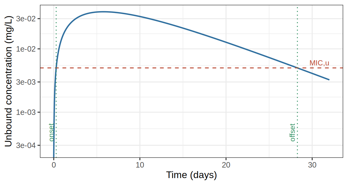
Worked example. For ka = 0.01/h, ke = 0.005/h, Vss = 50 L, targeting a continuous 28-day window with a single dose:

the smallest dose achieving this is 3.85 mg, with the window running from 0.28 to 28.28 days after administration:

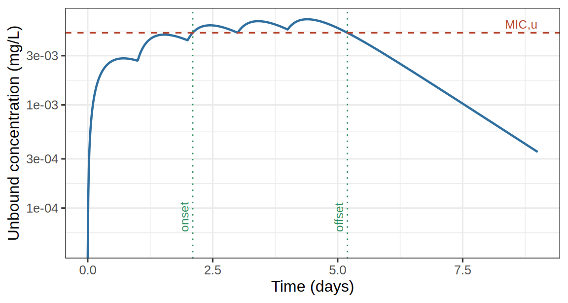
Why the onset can’t just be “the first time concentration crosses MIC_u”. With a faster, more slowly-accumulating regimen (ka = 0.1/h, ke = 0.03/h, Vss = 500 L, 5 daily doses), a slightly higher dose than the minimum can produce a brief early “blip”: right after the very first dose or two, concentration can poke above MIC_u for a short moment, well before the regimen has meaningfully accumulated - long before the real, sustained window later in the profile. Naively defining onset as “the very first crossing” breaks down here: as dose increases, that first crossing can jump backward to this tiny earlier blip, so the reported window’s duration stops increasing smoothly with dose and can drop sharply instead, making it impossible to solve for a well-defined minimum dose. Anchoring at the global peak and walking outward (the algorithm above) avoids this: a blip is only reachable by walking past a trough that has already dropped below threshold, so the walk-back stops at the real, sustained window’s onset instead. The Time to MIC,u column shown alongside each predicted dose is exactly this onset, for the rounded dose actually shown (formula_timeToMIC()) - the start of the window that actually delivers the requested coverage duration, not the onset of a blip that doesn’t:

This chapter’s \(h(t)\) is formula_doseKineticsShape(), the window-finding algorithm above is findWindow(), and the dose/time-to-MIC,u predictions are formula_doseMIC()/ formula_timeToMIC() - all in Resources/STATE_Objects.R. The same functions serve both the oral (multi-dose) and LAI (always a single dose) predictions, and the theoretical dose-landscape background grids described below.

3.3 Dose Rounding and Display

Predicted doses are rounded up to a practical value (never down, to avoid under-dosing): to the nearest whole mg for doses \(\geq 1\) mg, or to 2 significant figures below that. A dose beyond what the search considers practically achievable (1e9 mg) is treated as needing an effectively infinite dose rather than reported as a missing value, and displayed as the top dose category (“≥ 500 mg”/“≥ 1000 mg”, see below) both in the tables and in the dose-landscape plots.

3.4 Dose Landscape Plots

Each dose section also shows a dose landscape: a grid of theoretical doses computed across a wide range of hypothetical \(Vss_u\)/\(CL_{int,u}\) combinations (holding \(k_a\), \(F\), and the dosing regimen fixed at the values above), shaded by dose category. The two routes use different thresholds, shown in the footnote under each plot:

• Oral: green (\(\leq\) 100 mg, ideal for oral chemoprevention), yellow (101-499 mg, may be acceptable depending on overall profile and portfolio), red (\(\geq\) 500 mg).
• LAI: green (\(\leq\) 400 mg, meets the MMV criteria for late lead), orange (401-999 mg), red (\(\geq\) 1000 mg).

The compound’s own two predicted points (in silico and in vivo) are overlaid on this grid, making it easy to see how sensitive the predicted dose is to uncertainty in \(Vss_u\) or clearance. A compound whose Human CL,u or Vss,u falls outside the plotted range for a given Vss source is listed in a “Not shown” note under the plot rather than silently omitted.

The oral dose landscape additionally overlays diagonal elimination half-life reference lines (Chapter 2) - meaningful there because the oral terminal half-life is elimination-driven for the vast majority of compounds. The LAI dose landscape omits these lines, since the LAI terminal half-life is usually driven by the (fixed) absorption rate instead and would not track the plotted \(Vss_u\)/\(CL_{int,u}\) grid.

4 The Report

The Report button on the Unbound Parameters & Dose tab’s sidebar downloads a multi-sheet Excel workbook (.xlsx) documenting the uploaded inputs and every prediction shown in Chapters 2 and 3, for every compound currently loaded. This chapter describes what each of its 7 sheets contains. A report downloaded this way can itself be re-uploaded later on the File Input tab (Chapter 1), making it easy to resume a session or combine results across uploads.

Comparative User Inputs (below) is unchecked by default in the sidebar’s sheet selector - the other 6 sheets are included by default.

4.1 Unbound Parameters

One row per compound per Vss source (in silico / in vivo), exactly matching the on-screen Unbound parameters sub-tab: Compound, Vss source, Plasma Fu, TCGLS 3D7 IC50,u (nM), In vitro 48h PRR (log10), MIC,u (nM), Vss,u (L/kg), CLint,u (µL/min/mg microsome), Human CL,u (mL/min/kg), VLE (-log10 moles), and Zero CL dose (mg) - see Chapter 2 for how each of these is derived. A compound whose Zero CL dose is at or beyond the 1000 mg display cap is written as “≥ 1000 mg” text, matching the on-screen table, instead of the raw numeric placeholder value.

4.2 Oral Dose

One row per compound per Vss source, mirroring the on-screen Oral dose sub-tab: Compound (plain text here - the on-screen MMVSola link icon has no meaning in Excel), Vss source, Oral bioavailability (Fabs1), Absorption rate (1/hour), Absorption half-life (days), Elimination rate (1/hour), Elimination half-life (days), Terminal half-life (days), and “Oral dose for N days > MIC,u (mg)” - N being whatever MICu time (days) was set to when the report was generated. Doses at or beyond the 500 mg display cap are written as “≥ 500 mg” text, matching the app.

Below the table, the sheet embeds the same oral dose-landscape figure shown on screen, including its “Not shown” clause (listing any compound missing from the plot) and colour-scale legend as a footnote baked directly into the image.

4.3 LAI Dose

The long-acting-injectable equivalent of the Oral Dose sheet, one row per compound per Vss source: Compound, Vss source, LAI bioavailability (Fabs1), Absorption rate (1/hour), Absorption half-life (days), Elimination rate (1/hour), Elimination half-life (days), Terminal half-life (days), and “LAI dose for N days > MIC,u (mg)” (N = the sidebar’s MICu time selection, 90 or 180 days), with the same ≥1000 mg display-cap convention as the other dose sheet. The LAI dose-landscape figure and its footnote are embedded below the table in the same way as the Oral Dose sheet.

4.4 Science Cloud File

The raw, uncurated Science Cloud records behind every compound’s averaged input parameters - every row uploaded for every compound, stacked one compound after another. A record excluded from averaging via the File Input tab’s checkboxes (Chapter 1) is still listed here, but its row is shaded to flag that it was excluded. If a compound had no Science Cloud data uploaded for it (e.g. its parameters were entered entirely manually), it contributes no rows to this sheet.

4.5 User Inputs

One block per compound, each grouped into the same input categories shown in the app (e.g. Molecular Properties, Plasma Binding, Clearance) with one row per parameter: its inputted value, its validated value (after any range/consistency checks), unit, source (Science Cloud / user input / a previously uploaded report / a built-in default), and any validation note. This is the most granular sheet in the report - it is what a re-uploaded MMVFree report reads back to restore a session.

4.6 Comparative User Inputs

Unchecked by default. The same parameters as the User Inputs sheet, but reshaped so compounds run across columns instead of down separate blocks - one merged header row per compound, with Inputted/Validated/Source sub-columns beneath it - so that values for the same parameter across every loaded compound can be scanned side by side in a single row. Intended for comparing several candidate compounds at a glance rather than reviewing one compound’s full input record in detail (that’s what the User Inputs sheet above is for).

4.7 Additional Information

Two blocks, not tied to any particular compound: Constants - the fixed values used throughout the app’s calculations (e.g. reference body weight, MPPGL, liver weight, hepatic blood flow - see the Symbol Glossary in Chapter 2) - and Software versions, recording the exact MMVFree version and the versions of the underlying MMVshiny, MMVbase, MMVhuPKpred, and MMVhuPDpred packages used to generate this report, plus the report’s own User Inputs sheet format version (tracked separately from the app version, since other MMV apps such as MMVSola can import an MMVFree report).

References

Gabrielsson, Johan, and Dan Weiner. 2016. Pharmacokinetic and Pharmacodynamic Data Analysis: Concepts and Applications. 5th ed. Swedish Pharmaceutical Press.

Gibaldi, Milo, and Donald Perrier. 1982. Pharmacokinetics. 2nd ed. New York: Marcel Dekker.

Houston, J Brian. 1994. “Utility of in Vitro Drug Metabolism Data in Predicting in Vivo Metabolic Clearance.” Biochemical Pharmacology 47 (9): 1469–79.

Obach, R Scott. 1999. “Prediction of Human Clearance of Twenty-Nine Drugs from Hepatic Microsomal Intrinsic Clearance Data: An Examination of in Vitro Half-Life Approach and Nonspecific Binding to Microsomes.” Drug Metabolism and Disposition 27 (11): 1350–59.

Rowland, Malcolm, Leslie Z Benet, and Graham G Graham. 1973. “Clearance Concepts in Pharmacokinetics.” Journal of Pharmacokinetics and Biopharmaceutics 1 (2): 123–36.

Rowland, Malcolm, and Thomas N Tozer. 2022. Clinical Pharmacokinetics and Pharmacodynamics: Concepts and Applications. 5th ed. Lippincott Williams & Wilkins.